|
11 weeks
|
Corrected
|
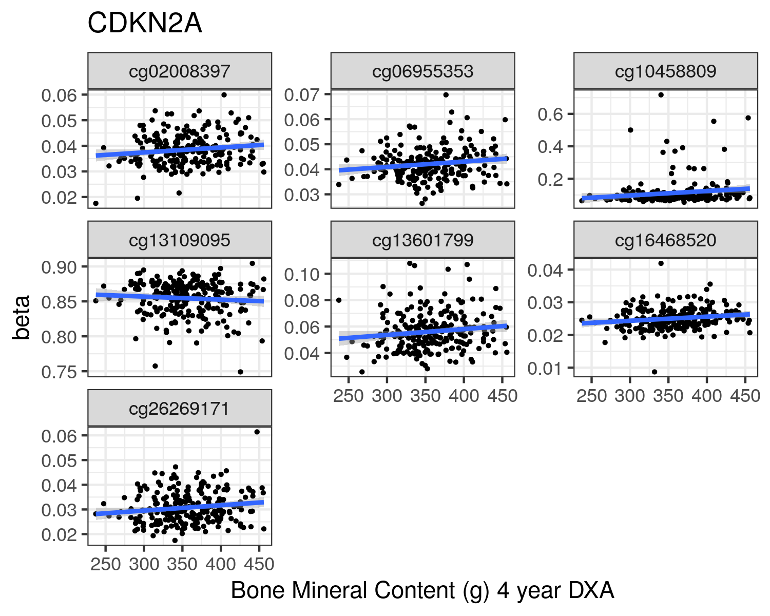
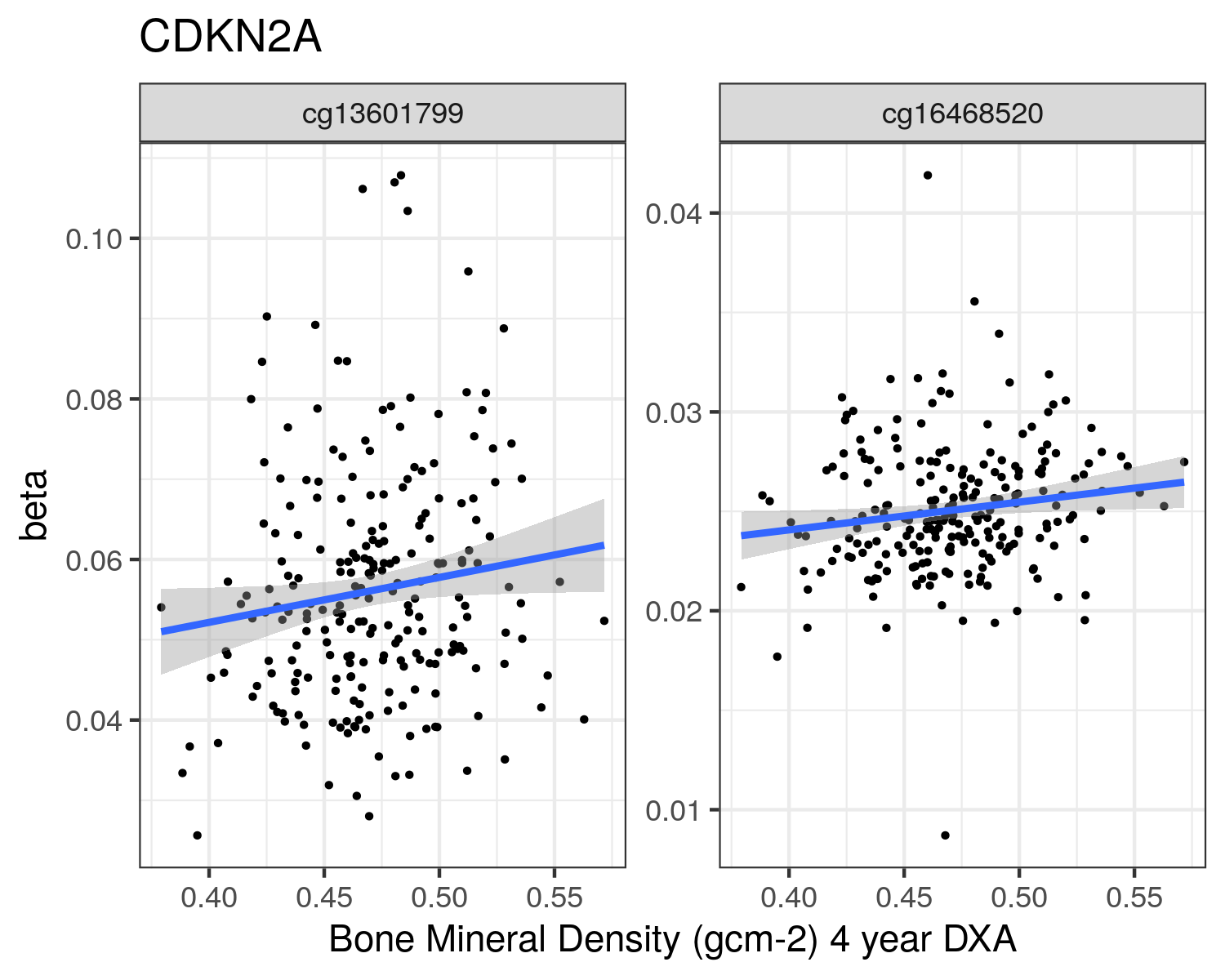
CDKN2A
|
Chr9: 21,968,233- 21,968,233
|
cg12840719
|
230.3170
|
0.0066
|
|
Chr9: 21,986,062- 21,986,062
|
cg00550721
|
-63.8120
|
0.0291
|
|
Chr9: 21,991,666- 21,991,666
|
cg13109095
|
-122.1244
|
0.0358
|
|
Chr9: 21,975,898- 21,975,898
|
cg10458809
|
27.5771
|
0.0365
|
|
Chr9: 21,971,256- 21,971,256
|
cg08686553
|
96.1148
|
0.0378
|
|
Uncorrected
|
Chr9: 21,968,233- 21,968,233
|
cg12840719
|
180.7349
|
0.0147
|
|
Chr9: 21,986,062- 21,986,062
|
cg00550721
|
-50.0384
|
0.0411
|
|
Corrected
|
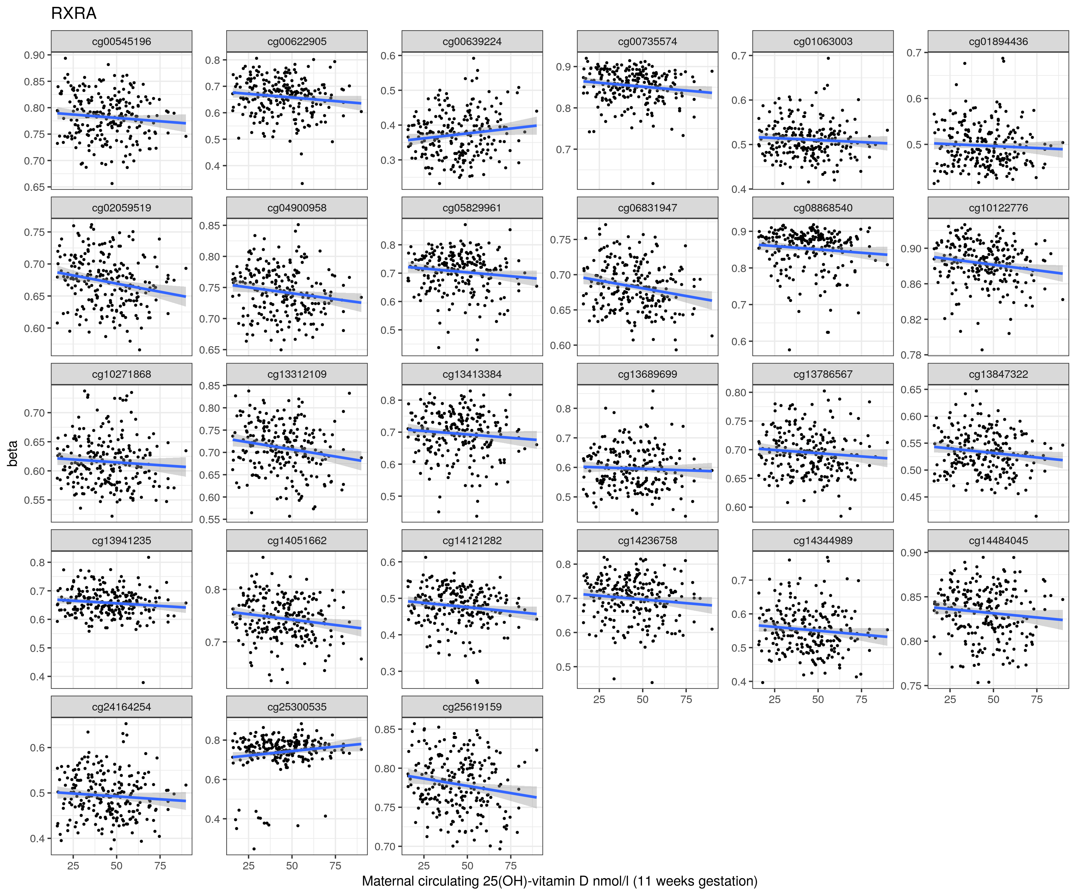
RXRA
|
Chr9:137,329,237-137,329,237
|
cg14344989
|
-92.4988
|
0.0005
|
|
Chr9:137,250,935-137,250,935
|
cg02059519
|
-106.0882
|
0.0007
|
|
Chr9:137,271,457-137,271,457
|
cg13312109
|
-74.2411
|
0.0007
|
|
Chr9:137,263,644-137,263,644
|
cg05829961
|
-106.9248
|
0.0019
|
|
Chr9:137,283,224-137,283,224
|
cg00622905
|
-108.5121
|
0.0021
|
|
Chr9:137,260,147-137,260,147
|
cg04900958
|
-99.1450
|
0.0033
|
|
Chr9:137,268,524-137,268,524
|
cg10122776
|
-141.6744
|
0.0035
|
|
Chr9:137,266,722-137,266,722
|
cg06831947
|
-109.8622
|
0.0036
|
|
Chr9:137,279,180-137,279,180
|
cg14051662
|
-82.8152
|
0.0040
|
|
Chr9:137,262,485-137,262,485
|
cg25619159
|
-90.9658
|
0.0043
|
|
Chr9:137,329,341-137,329,341
|
cg24164254
|
-88.6921
|
0.0068
|
|
Chr9:137,282,509-137,282,509
|
cg00735574
|
-95.1502
|
0.0105
|
|
Chr9:137,301,743-137,301,743
|
cg08868540
|
-130.8756
|
0.0105
|
|
Chr9:137,302,231-137,302,231
|
cg13413384
|
-92.9525
|
0.0107
|
|
Chr9:137,252,129-137,252,129
|
cg14236758
|
-89.7349
|
0.0114
|
|
Chr9:137,326,382-137,326,382
|
cg25300535
|
27.8782
|
0.0142
|
|
Chr9:137,271,104-137,271,104
|
cg01894436
|
-96.1754
|
0.0225
|
|
Chr9:137,272,766-137,272,766
|
cg13847322
|
-73.9350
|
0.0230
|
|
Chr9:137,299,685-137,299,685
|
cg00545196
|
-63.1364
|
0.0282
|
|
Chr9:137,268,074-137,268,074
|
cg14121282
|
-65.2194
|
0.0323
|
|
Chr9:137,257,228-137,257,228
|
cg10271868
|
-62.4176
|
0.0361
|
|
Chr9:137,298,350-137,298,350
|
cg01063003
|
-71.8198
|
0.0376
|
|
Chr9:137,258,920-137,258,920
|
cg13786567
|
-63.6464
|
0.0397
|
|
Chr9:137,265,865-137,265,865
|
cg14484045
|
-77.6335
|
0.0440
|
|
Chr9:137,270,186-137,270,186
|
cg13941235
|
-44.6552
|
0.0466
|
|
Chr9:137,225,311-137,225,311
|
cg13689699
|
-49.7538
|
0.0487
|
|
Uncorrected
|
Chr9:137,266,722-137,266,722
|
cg06831947
|
-93.4263
|
0.0020
|
|
Chr9:137,250,935-137,250,935
|
cg02059519
|
-79.0829
|
0.0022
|
|
Chr9:137,271,457-137,271,457
|
cg13312109
|
-50.1030
|
0.0066
|
|
Chr9:137,268,524-137,268,524
|
cg10122776
|
-108.6295
|
0.0122
|
|
Chr9:137,262,485-137,262,485
|
cg25619159
|
-71.3247
|
0.0135
|
|
Chr9:137,279,180-137,279,180
|
cg14051662
|
-62.6430
|
0.0146
|
|
Chr9:137,260,147-137,260,147
|
cg04900958
|
-63.4042
|
0.0187
|
|
Chr9:137,326,382-137,326,382
|
cg25300535
|
24.7823
|
0.0230
|
|
Chr9:137,282,509-137,282,509
|
cg00735574
|
-56.3782
|
0.0273
|
|
Chr9:137,268,074-137,268,074
|
cg14121282
|
-43.7701
|
0.0299
|
|
Chr9:137,221,918-137,221,918
|
cg00639224
|
32.4576
|
0.0406
|
|
Chr9:137,272,766-137,272,766
|
cg13847322
|
-53.5243
|
0.0433
|
|
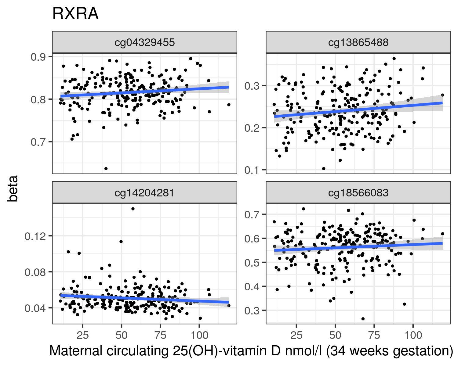
34 weeks
|
Corrected
|
CDKN2A
|
Chr9: 21,975,622- 21,975,622
|
cg25339269
|
-472.4791
|
0.0081
|
|
RXRA
|
Chr9:137,217,473-137,217,473
|
cg14204281
|
-258.5922
|
0.0259
|
|
Chr9:137,301,635-137,301,635
|
cg18566083
|
114.9198
|
0.0483
|
|
Chr9:137,215,364-137,215,364
|
cg04329455
|
99.9363
|
0.0489
|
|
Uncorrected
|
Chr9:137,299,285-137,299,285
|
cg13865488
|
59.8832
|
0.0427
|
![Overall Fracture Incidence Increases With Age Data from 5 million adults in the General Practice Research Database 1988-1998. A Incidence of all fractures at any site by sex and age. B Fractures by sex and age at select sites, pelvis, Femur/Hip & Vertebra confer the greatest increased mortality rates and Radius/Ulna has the greatest sexual dimorphism. (Adapted from van Staa et al. [238].)](figs/adapted_from_VanStaa2001_Fig1-2.png)
![Bone Mass Over The Lifecourse Bone mass increases from intrauterine development through to a peak in early adulthood. Intervention in early life to modulate growth trajectory and increase peak mass may provide a higher starting point and delay bone loss in later life. (Reproduced from [245].)](figs/Harvey2014bfig1.png)